timeshift(shifts, set[])

The timeshift function produces a set of series, each shifted in time by a set of defined offsets. The second argument to timeshift is a series set, typically a composite metric query. Timeshift will execute the composite set for each timeshifted interval.

The first argument to timeshift is a comma-separated list of offsets that adjust the start time of the query. The format for time shifts are:

"<number>[,<number>,...][period abbreviation]"

Time shifts are considered to be relative to the current time set by the start_time= parameter of the API query and are implied to be a negative time shift unless specified otherwise (a timeshift of “7d” and “-7d” are the same). You can specify a forward shift by adding the plus sign in front of the shift parameter, so “+7d” means shift one week into the future. Time shifts periods are specified with a time period abbreviation. The list of defined time period abbreviations are listed in the next section. The returned series are in the same order as the order of the time shifts.

Given this is relative to current time, a time shift of “0” implies no shift at all, so:

timeshift("0w", set[]) == set[]

A time shift of “1” implies a shift one period back, so in the example below one series is returned timeshifted one week back:

timeshift("1w", set[])

A timeshift with multiple shifts will return the series in the order they are listed. So the following query returns two series: the current series and the same function timeshifted one week back, in that order.

timeshift("0,1w", set[])

You can place the zero shift (current series) later in the list too:

timeshift("1,0w", set[])

Is the same query as before, but the returned series are in the opposite order.

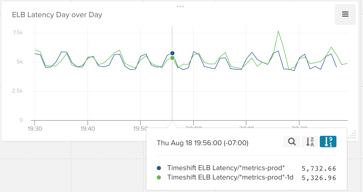
Example

This example shows how to create a graph with two lines for the max values of the AWS.ELB.Latency metric across all measurements that include the tag “host:metrics-prod”.

timeshift("0,1d",max(series("AWS.ELB.Latency",{"host":"*metrics-prod*"},{function:"sum"})))

The two series are the timeshifted by one day.

Response time modification

In order for the returned time series to plot correctly (and work in subsequent time series transforms), the measure_time’s of a timeshift time series will be adjusted to the current time span by adding the time shift duration to the measure time. Therefore, the measure_times of a “-7d” timeshift will be adjusted using: measure_time + 7d.

Each time shifted series will include the time shift offset in the returned series object with the key name timeshift.

End of time implications

The end of a time shifted series will only extend to minimum(time_shift_duration, (end_time-start_time)). Therefore, given a time shift of “0,-7d” the “-7d” shifted series will extend up to min(7d, (end_time-start_time)). This means that if start_time=now-1day, then the -7d shifted series will be a single series from one day, 7 days ago since (end_time(now) - start_time) => 1 day.

The max span is defined by the smallest time shift. Therefore, with a time shift of “0,1,2w” you will get 3 series: one for the current week and two for the two previous weeks and each series will be one week long.

Timeshift period abbreviations

Abbreviations are case insensitive.

Abbreviation	Period
s	Second
min	Minute
h	Hour
d	Day
w	Week
mon	Month (30 days)
m	UNUSED (not valid and will return an error)

Note

Due to composite metrics currently being limited to alerting on the past 60 minutes of data (see Alerts on Composite Metrics), the timeshift function will only be able to be evaluated properly if data points are rendered in 60 minute window. Therefore, alerting on the timeshift function requires that the period is set to a minimum of 60 seconds, and in the case you are using timeshift for data 1 week or older you will need to set the period to 900 seconds.

Example:

timeshift("0,1w", s("foo.total", {"host":"*"}, {period:"900"}))